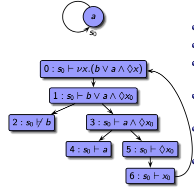
Well, the loops in the proof trees in local model checking are always worth a discussion, even though everything is found on the slides, so that I just cite the related slides below and comment on them. Have a look at the example below where we just have a transition system with a single state where "a" holds, but "b" is false (taken from slide 107 of the mu-calculus chapter).

The proof tree for the formula nu x.(b | a&<>x) is shown above and as can be seen, it has a loop. Note that the formula is equivalent to the CTL formula E[a WU b] and that the least fixpoint mu x.(b | a&<>x) is equivalent to the CTL formula E[a SU b] (note that the Kripke structure has no deadend states which simplifies these equivalences).
Using global model checking (or just reasoning with the semantics of the formulas), we can see that E[a WU b] holds on the state while E[a SU b] does not hold there: For the weak until, it is allowed to always have "a" true and never reach a state where "b" holds, but the strong until demands that a state where "b" holds is finally reached and until that time, only states where "a" holds must be visited.
However, the equivalent mu-calculus formulas nu x.(b | a&<>x) and mu x.(b | a&<>x) generate similar proof trees (but the result for the least fixpoint is different!). Hence, we must read that proof tree differently for least and greatest fixpoint formulas.
As explained on slide 108, states closing a loop satisfy greatest but not least fixpoint formulas. Slide 109 explains why that is so, and to keep the story short: for least fixpoints, we try to choose as few states as possible to satisfy them, while for greatest fixpoints, we try to choose as many states as possible to satisfy them. In case of loops, we have the freedom to choose, since those states satisfy the fixpoint equation.